Weight decay has a direction, too
When we tune weight decay, we usually tune its strength: how large should the coefficient be, should it change during training, and should different modules use different values? These questions all assume that the direction of decay is already settled. For matrix weights, it need not be.
AdamW separates the task update from weight shrinkage. The optimizer follows information from gradients; the decay term acts on the current weights. Ordinary weight decay (WD) points along , but a matrix’s singular-value decomposition gives us other directions to consider.
On its own, ordinary WD makes every singular value smaller by the same factor. The matrix shrinks, but its relative spectrum stays the same. Can we instead choose which parts of the spectrum to shrink more strongly?
Spectral-power weight decay, denoted by WD, makes this choice through a singular-value power. Let have the compact rank- SVD , where have orthonormal columns and are the nonzero singular values. Define
The exponent determines how shrinkage varies with mode size. We use for the decay direction and WD for the method. The associated penalty is
Here is the Schatten norm. For , ; at , is a nuclear-norm subgradient (Lewis, 1995; Watson, 1992). Ordinary WD is recovered at . Other powers change the relative pressure on the large and small singular values—the head and tail of the spectrum.
The next question is whether changing the weight spectrum also changes the representations the model learns, and whether those changes help prediction. We will follow this progression from a solvable linear model to Transformer experiments.
The weight spectrum tells us how parameter magnitude is distributed across singular modes. The activation spectrum tells us what representations those weights produce on the data. Validation loss measures how well the resulting model predicts.
These are related measurements, not interchangeable ones. WD acts on weights rather than the current task gradient, so a change in rank is evidence of a geometric effect—not, by itself, evidence of better learning.
1. From ordinary weight decay to decoupled optimizers
1.1 When L2 regularization and weight decay coincide
Ridge regression and Tikhonov regularization add a quadratic penalty to control parameter size (Hoerl & Kennard, 1970; Tikhonov & Arsenin, 1977):
Let be the task loss, the L2 penalty coefficient, the base step size, and a schedule multiplier. In plain SGD, the update is
Thus, L2 regularization and weight decay give the same plain-SGD update when . The penalty controls total squared weight magnitude, which can also be written as
Early analyses of weight decay studied how this norm penalty suppresses irrelevant components and limits the effect of noise in the training targets (Krogh & Hertz, 1991).
1.2 Why the distinction matters beyond plain SGD
Momentum averages gradients over time (Sutskever et al., 2013); AdaGrad and Adam also rescale coordinates using gradient history (Duchi et al., 2011; Kingma & Ba, 2015). Write the parameters as a vector , the stochastic task gradient as , and the preconditioner as . In Adam, the diagonal scaling uses the inverse square root of a second-moment estimate, with a numerical stabilizer. Leaving out momentum averaging for the moment, coupled L2 regularization has the schematic form
Decoupled decay instead acts directly on the parameters:
For plain SGD, , and matching recovers the equivalence above. In Adam, a coupled L2 term also enters the moment estimates and is transformed by the preconditioner. Moving it outside the optimizer therefore changes the algorithm, not just the notation. This distinction can also affect generalization (Tang et al., 2025; Zou et al., 2023).
1.3 A separate branch for decay
AdamW makes this separation explicit (Loshchilov & Hutter, 2019). Throughout the article, we write the decoupled update as
Here is the task direction computed from the gradient and optimizer state. The base coefficients and are fixed; schedules both terms. “Decoupled” means that decay bypasses the optimizer’s preconditioning and state updates. It does not require the two terms to have separate schedules.
Much of the work on this branch concerns decay strength. AdaDecay assigns parameter-wise rates using gradient statistics (Nakamura & Hong, 2019). Adaptive WD adjusts coefficients according to the relative strengths of task and L2 updates (Ghiasi et al., 2023). AlphaDecay assigns module-wise coefficients in LLMs to balance heavy-tailed spectral statistics (He et al., 2025).
These methods refine how much decay to apply and where to apply it. Parameter-wise scaling can itself change the update’s geometry, so strength and direction are not completely separate. Our question is more specific: can we prescribe shrinkage in the weight matrix’s singular basis?
1.4 Matrix-aware optimizers make geometry explicit
K-FAC, Shampoo, SOAP, and Muon already use matrix structure to shape task updates (Gupta et al., 2018; Jordan et al., 2024; Martens & Grosse, 2015; Vyas et al., 2025). Muon offers a particularly simple example: its idealized matrix update preserves the singular directions of a momentum matrix while replacing each nonzero singular value by one (Jordan et al., 2024). Polar Express efficiently approximates this polar-factor computation (Amsel et al., 2026).
The same kind of matrix operation can be useful in the decay branch, but it acts on a different object. Muon transforms task momentum; WD transforms the current weights. One chooses how to follow the task signal, the other how to regularize the parameters.
2. What ordinary weight decay controls
2.1 Isolated decay changes scale, not normalized shape
Set the task update aside. For nonzero , with , an ordinary-WD step gives
where is the current schedule multiplier and . It follows that
Both the spectral and Frobenius norms shrink, but all singular-value ratios remain unchanged. So do stable rank and entropy effective rank, or eRank, defined below. This is a statement about an isolated decay step. During training, task updates also change singular values and singular vectors; decay can influence the final spectrum through its interaction with those updates (Loshchilov & Hutter, 2019).
2.2 Norm control can still affect learned structure
Ordinary WD can therefore be associated with low-rank structure even though its isolated step preserves spectral ratios. Its interaction with optimization has several mechanisms (Zhang et al., 2019). Factorization adds another: the model may depend on a product of weights rather than either factor alone. For query and key weights , write . When the factor dimensions are large enough to represent , the classical identity is (Srebro et al., 2004)
Here is the nuclear norm, and the minimum is over compatible factors . This connects quadratic penalties on factors to a low-rank preference for their product. The minimization matters: arbitrary factors encountered during training need not attain it. Analyses of low-rank attention likewise require specific balance and dynamics conditions (Kobayashi et al., 2024).
Weight norms also affect effective step size. In a scale-invariant parameterization, rescaling the weights changes how much a given update moves the represented function (van Laarhoven, 2017). Hyperball addresses this directly by controlling the Frobenius norms of both weights and optimizer updates (Wen et al., 2026). For a small task step, the angular displacement in parameter space is approximately
The component is tangent to the weight sphere, and . When the task direction has a controlled norm, serves as a proxy for the effective learning rate (ELR). Thus, changing weight scale can change learning dynamics even without directly changing spectral shape.
2.3 Reading the spectrum: notation and rank metrics
For nonzero , order the singular values as , where includes zero modes. Define and, for a probability vector , , with . The spectral norm is . In the table, is the number of leading modes retained, and normalized entropy assumes .
| Metric | Definition | Interpretation |
|---|---|---|
| Algebraic rank (Higham, 2002) | Number of nonzero | Exact dimension of the active subspace |
| Stable rank (Sanyal et al., 2020) | Total squared energy relative to the largest mode | |
| Entropy effective rank, or eRank (Roy & Vetterli, 2007) | , | Effective number of modes carrying singular-value mass |
| Output-energy effective rank (Roy & Vetterli, 2007) | , | Effective number of energy-bearing output modes under isotropic input |
| Top- energy (Eckart & Young, 1936) | Concentration of energy in the leading modes | |
| Normalized spectral entropy (Shannon, 1948) | Entropy relative to a uniform spectrum |
Stable rank and eRank both ignore overall scale, but they summarize the spectrum differently. Stable rank compares total squared energy with the largest mode; eRank measures how evenly singular-value mass is distributed. Output-energy effective rank instead uses squared singular values. None of these is attention entropy, which is computed from post-softmax attention probabilities (Roy & Vetterli, 2007; Vaswani et al., 2017; Zhai et al., 2023). Below, “rank” refers to the named statistic, not necessarily algebraic rank.
3. Spectral-power weight decay: direction, theory, and spectrum shaping
3.1 Definition and associated penalty
To move beyond equal relative shrinkage, replace each singular value in the decay direction by a power:
Three useful cases are
At , this is ordinary WD. At , the active polar factor assigns the same absolute decay to every nonzero mode. At , large modes receive more decay in both absolute and relative terms. Zero modes contribute zero to , consistent with the active polar factor and the nuclear-norm subdifferential (Cai et al., 2010; Higham, 1986; Watson, 1992).
For , this direction is the gradient of a unitarily invariant penalty:
The exponent in the direction is , whereas the Schatten penalty has order (Lewis, 1995). At , the penalty is the nonsmooth nuclear norm, and is one of its subgradients (Cai et al., 2010; Watson, 1992). This case is also studied as a way to encourage low-rank weights (Andriianov et al., 2026).
We apply the direction through the decoupled update
We keep the same convention for fixed base coefficients and the shared schedule. A practical point is worth emphasizing: changing changes both the norm of and how that norm is distributed across modes. Equal numerical values of do not match decay strength across powers.
3.2 Computing WD
For integer , the direction can be computed without an SVD. Let and be the output and input dimensions, choose the smaller Gram matrix, and write the active polar factor as . For any nonnegative integer ,
These identities are exact. In practice, we approximate with Polar Express (Amsel et al., 2026).
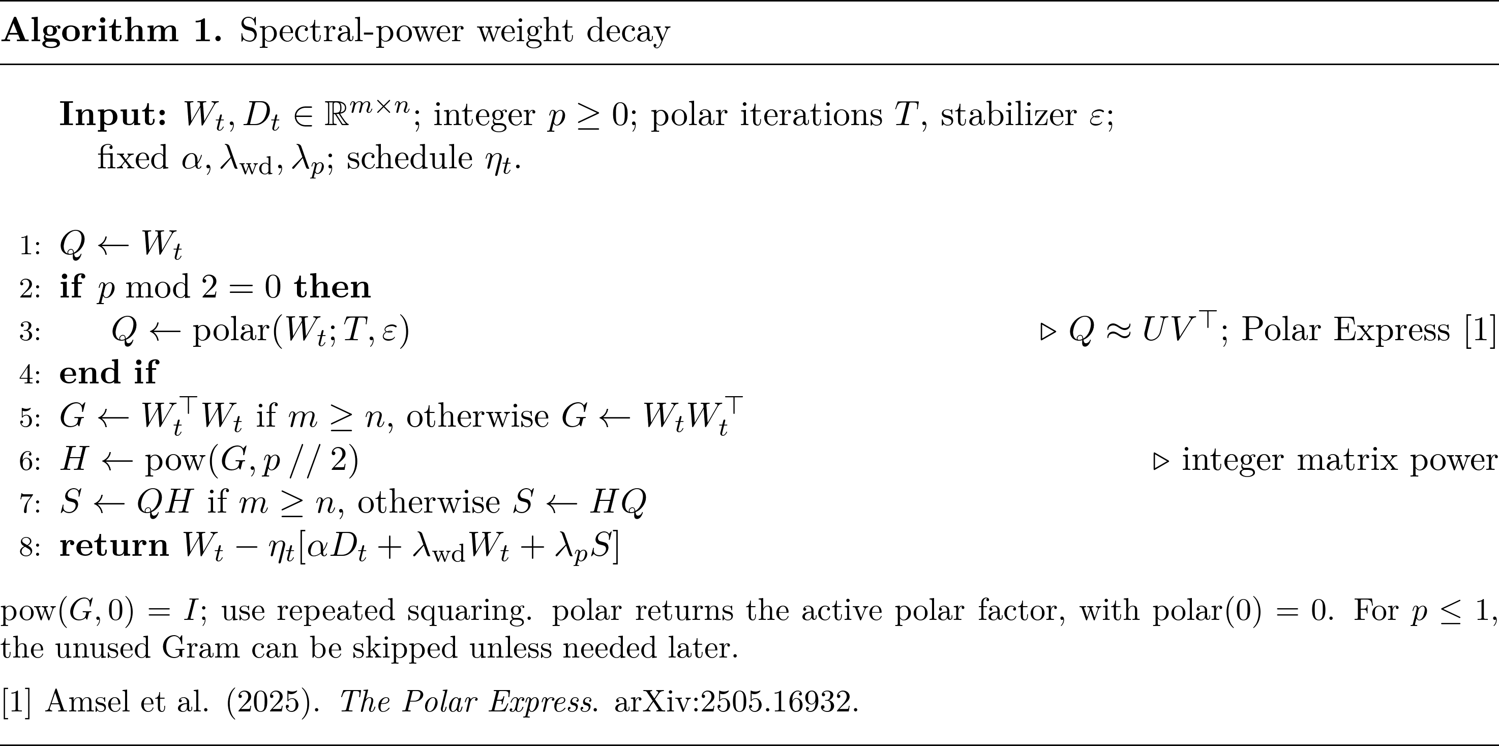
Algorithm 1. Computing spectral-power weight decay with a smaller Gram matrix and a polar-factor approximation. Odd powers need only matrix products; even powers also use Polar Express. The final line allows ordinary WD and the spectral term to be used together.
There is no need to form a Gram matrix at or . For larger powers, repeated squaring reuses intermediate results—for example, . The cost depends on matrix shape, exponent, and the number of polar iterations; avoiding an SVD does not make the extra decay term free. The check below uses eight Polar Express iterations, denoted PE8.
PE8 versus SVD: a small-matrix implementation check
We tested FP32 PE8 on full-rank , , and matrices with log-spaced singular values and seeds 42–44. Write the condition number as . The eight quintic coefficient sets use the Polar Express construction with design lower bound and safety scaling 1.01. The reference is an FP64 SVD of the same FP32 input. Each entry reports the largest relative Frobenius error, , across the nine shape/seed combinations.
At , the algorithm returns directly. At condition number , many normalized singular values lie below the polynomial schedule’s design interval. Eight iterations cannot accurately recover these modes in the equally weighted polar direction, giving a large error at . Their contribution to and , however, is downweighted by . The small errors in those columns therefore indicate an accurate decay direction in relative Frobenius norm, not accurate recovery of every singular mode.
3.3 Pure decay: separating scale from shape
Start with decay alone. Let continuous time represent cumulative schedule time, , and set . Since decay preserves singular directions, each positive singular value follows
For an initially positive mode, the solutions for the powers used below are
The relative shrinkage rate makes the difference between powers especially clear:
At , every mode loses the same fraction of its size. For , large modes shrink faster in relative terms, so the normalized spectrum flattens. For , small active modes shrink faster in relative terms and can reach zero in finite continuous time.
The continuous flow should not be confused with a finite explicit step. At , the positive-part solution has the same form as nuclear-norm proximal soft-thresholding (Cai et al., 2010; Parikh & Boyd, 2014). But an explicit polar step that crosses zero produces , rather than clipping the mode to zero. For the explicit method, “tail suppression” is therefore more precise than claiming automatic rank truncation.
While ,
Only at is the relative Frobenius contraction rate independent of the current spectrum.
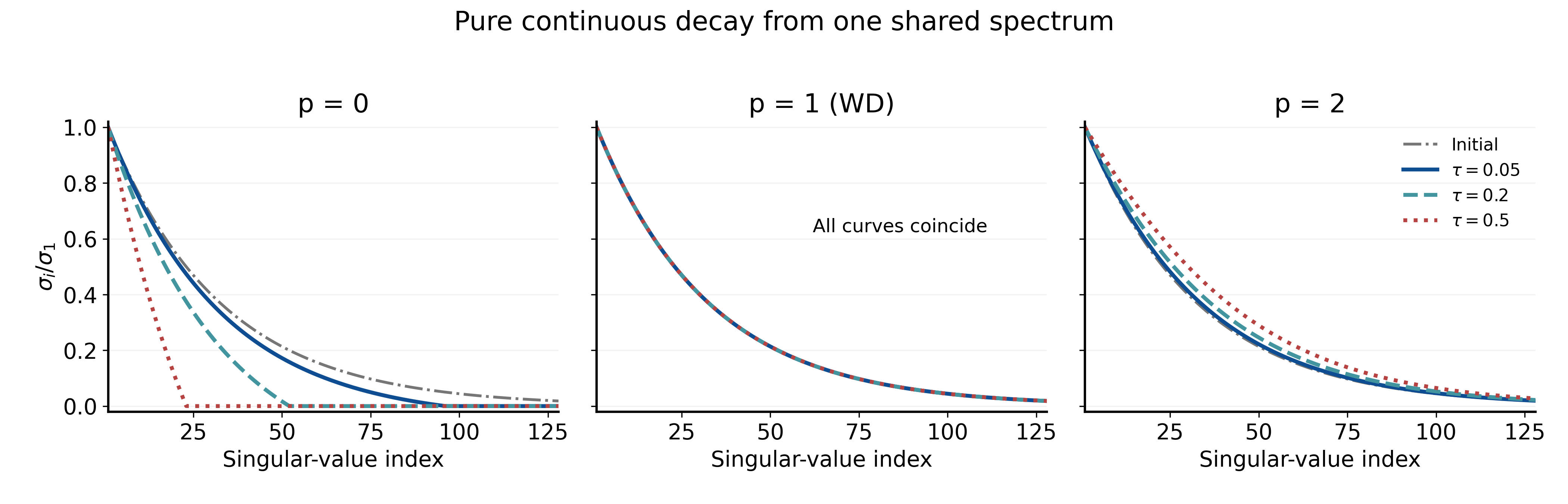
Figure 1. Pure continuous decay from a shared initial spectrum, at different cumulative decay exposures . Each curve is normalized by its current largest singular value. At , small modes reach zero first; at , all normalized curves coincide; at , the relative spectrum becomes flatter.
The upward movement of the normalized curves does not mean that any singular value grows. Every active mode is shrinking; the largest one simply shrinks proportionally faster. This distinction will matter when we compare trained models.
Pure decay can also approximate a local segment of training when . A falling learning rate alone does not imply this condition: the task and decay terms share the same multiplier .
The coefficient can change shape, too. For one explicit step, let and , the relative decay applied to the leading mode. If the step preserves signs and ordering,
For , the derivative is zero at , positive for , and negative for . The exponent determines the direction of the shape change; the coefficient determines how far the step moves in that direction. Ordinary WD is the special case in which changing isolated decay strength leaves normalized shape untouched.
3.4 A linear toy model: from weight spectra to output spectra
We can now add a fitting objective and solve for the resulting spectrum. Let the dense teacher be , with singular values . Consider
Here is a coefficient in the objective; for plain gradient descent, it corresponds to in our update notation. The trace inequality allows the optimum to be chosen with the teacher’s singular vectors (Lewis, 1995). The squared error is strongly convex and the spectral penalty is convex, so the optimal matrix is unique. Its singular values solve the scalar problems (Parikh & Boyd, 2014)
Ordinary WD gives at , scaling all teacher modes equally. For and ,
so large teacher modes are compressed more strongly in relative terms. At , the scalar equation again has a unique nonnegative root. At , the solution is singular-value soft-thresholding (Cai et al., 2010). These are different spectral responses to the same fitting task.
We verify the solutions with plain gradient descent, using a proximal step at . Whitened inputs then let us check exactly how the learned weight spectrum appears in the outputs.
Finite-sample check. We construct paired positive/negative samples in dimension . Reduced QR yields a centered design satisfying
to a maximum absolute error of ; the largest absolute coordinate mean is . The non-diagonal teacher has singular values , and we use . This construction gives an exactly whitened finite-sample input up to numerical precision (Kessy et al., 2018).
The optimized singular values closely match the analytic values :
| Analytic singular values | Covariance–SVD identity error | ||
|---|---|---|---|
| 0 | |||
| 1 | |||
| 2 | |||
| 4 |
The last column checks a separate identity. Since the output matrix is centered,
Thus, the nonzero covariance eigenvalues are , while the singular values of are . This identity holds for any under these inputs; it is distinct from the preceding column’s check that optimization reached the analytic solution.
From the solution to the solution, output-energy effective rank rises from to , and activation eRank rises from to . Both reflect a less concentrated spectrum, but the former weights modes by squared singular values and the latter by singular values.
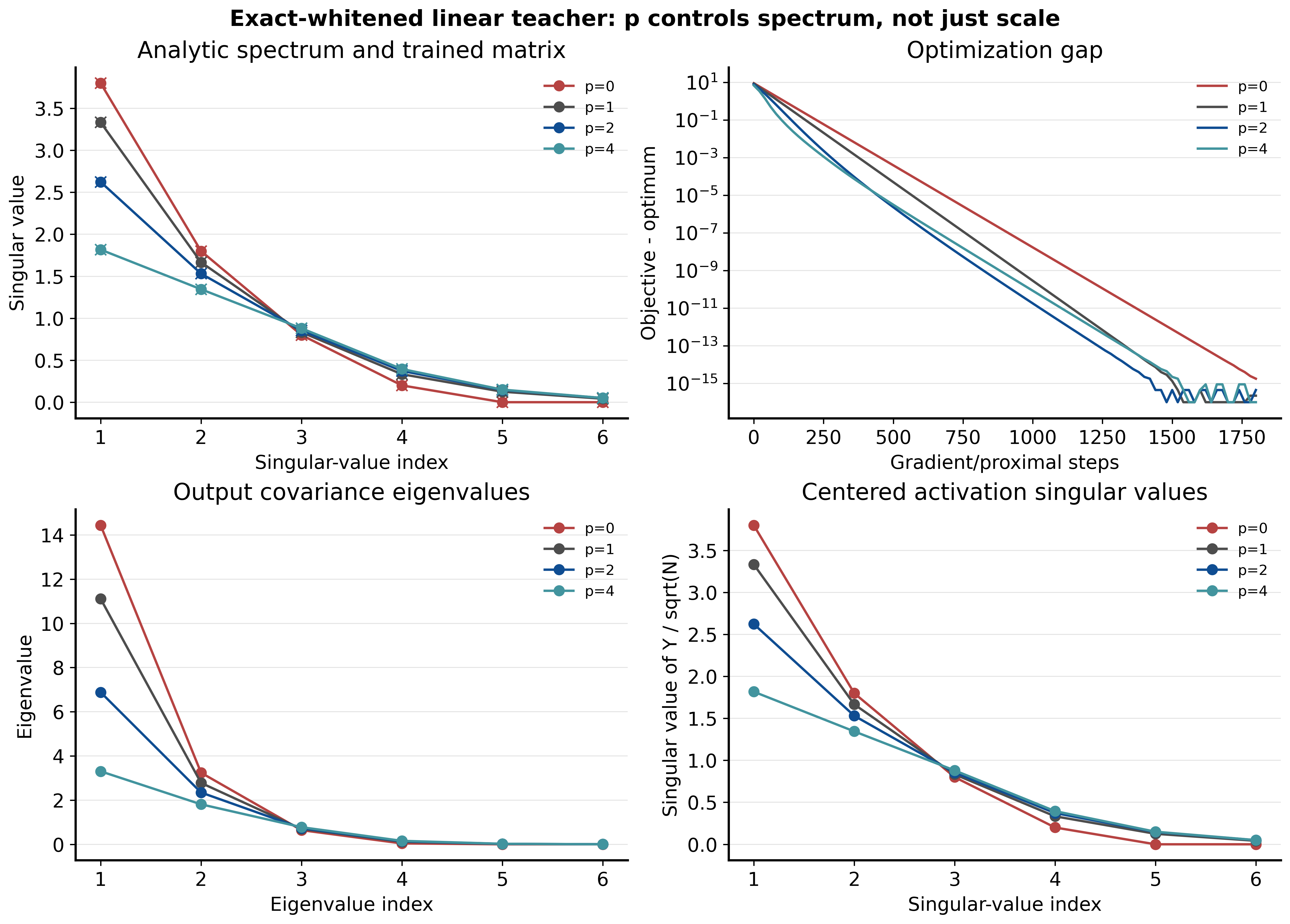
Figure 2. The linear teacher experiment. Top left: analytic and optimized weight spectra. Top right: each run’s regularized objective minus its own optimum. Bottom left: output-covariance eigenvalues. Bottom right: singular values of the centered outputs divided by .
The agreement between the top-left and bottom-right panels is a consequence of whitening, not an additional empirical correlation. The optimization-gap panel rules out incomplete convergence as the explanation for the different endpoint spectra; it does not compare a common unregularized loss across powers.
For general centered inputs with covariance , the output covariance is , rather than . The input spectrum and its alignment with the weight’s singular vectors then matter as well. This is why the clean weight-to-activation correspondence here should not be assumed in a Transformer.
3.5 An eight-layer Transformer: does the spectral effect survive training?
We next compare in an 8-layer, width-512 SwiGLU Transformer. We first hold the decay coefficient fixed, then sweep it separately for each power.
Varying the power. How does the spectrum change beyond the leading mode?
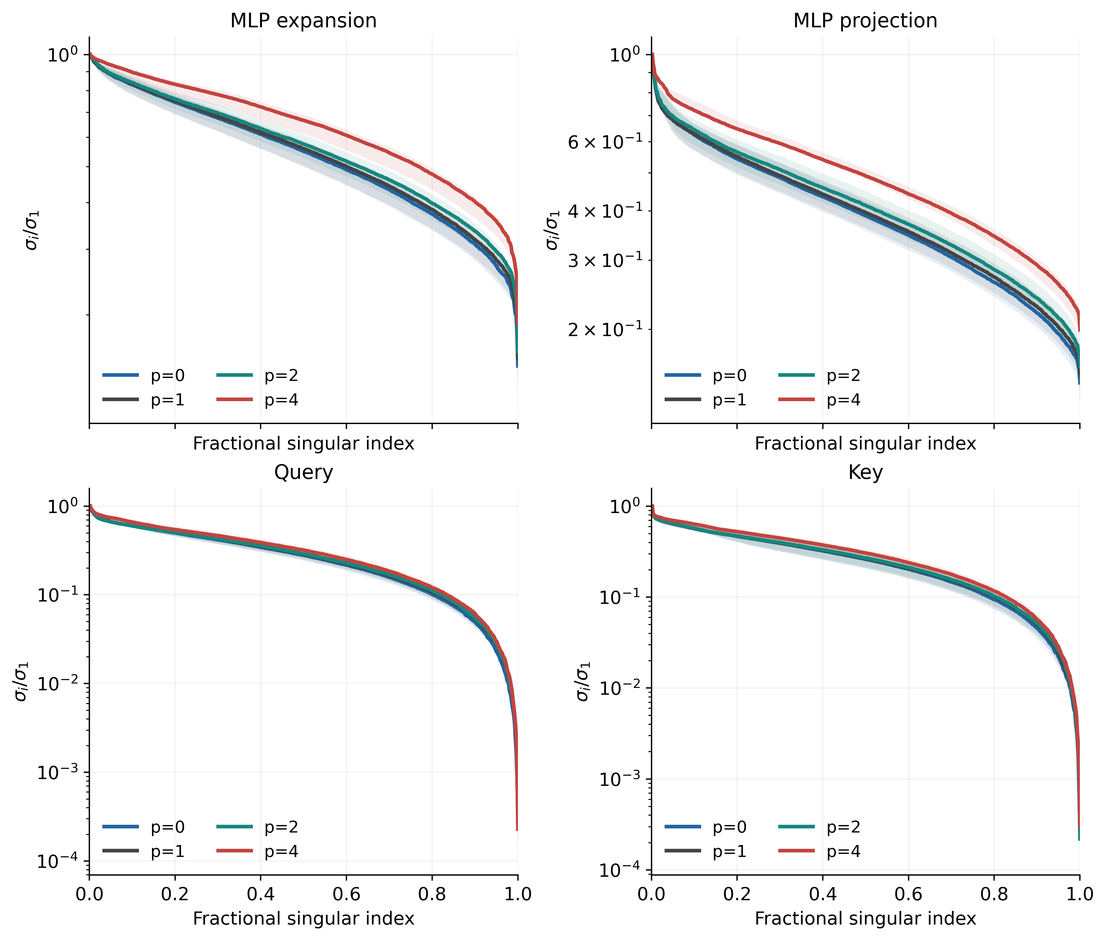
Figure 3. Normalized weight spectra for the eight-layer Transformer. Lines show the median across layers; shading shows the 25th–75th percentiles across layers. The horizontal axis is fractional singular-value index, and the vertical axis is .
The clearest separation is at , especially in the MLP expansion and projection matrices. More of their spectrum remains large relative to the leading mode. Q and K show much smaller differences, with the curves largely overlapping. The pure-decay tendency is still visible after training, but its magnitude depends strongly on the matrix family.
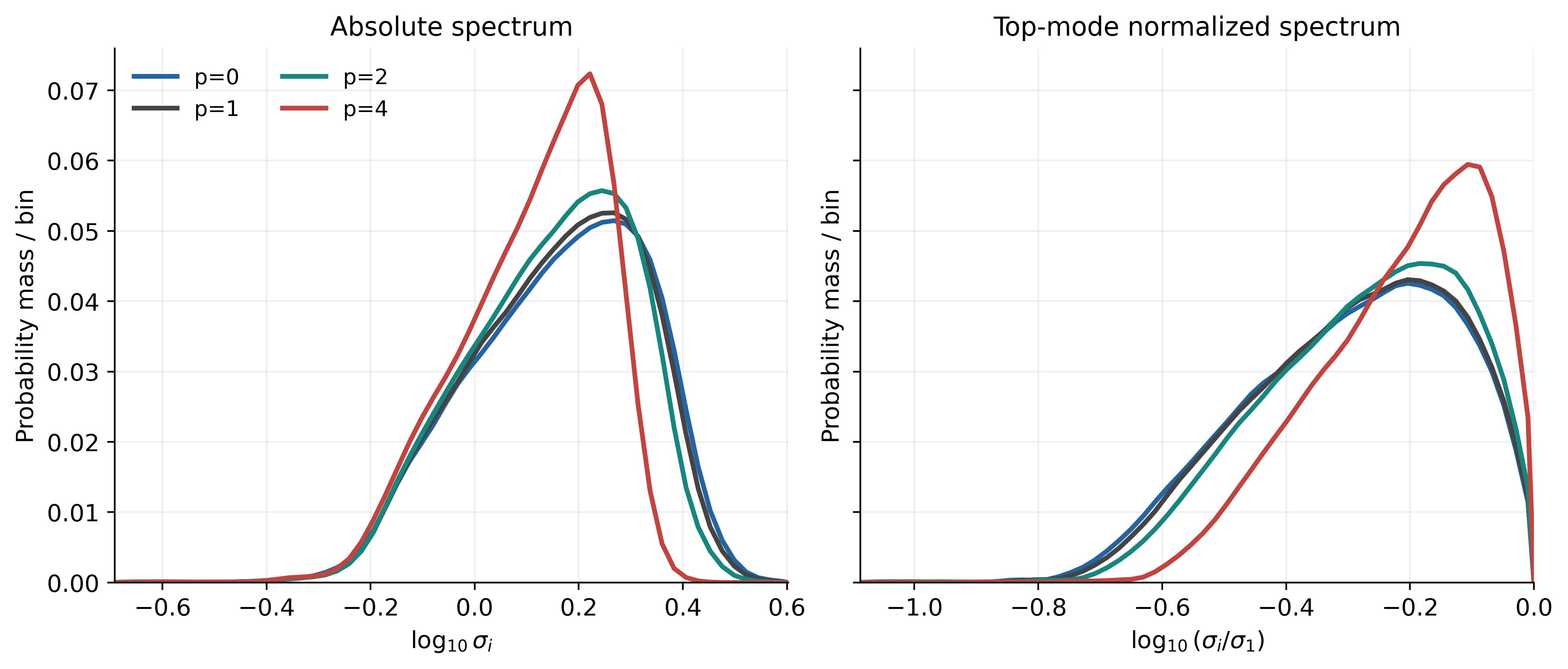
Figure 4. Spectral distributions of the eight MLP expansion matrices. Left: . Right: , using each matrix’s own largest singular value. Each matrix contributes equal probability mass. The vertical axis is mass per bin; smoothing is only for display.
The two panels separate absolute size from relative concentration. At , the upper end of the absolute spectrum moves left, while the normalized bulk moves toward zero—that is, toward . A flatter normalized spectrum can therefore come from suppressing the head, without increasing the absolute size of the other modes. The taller peak indicates that mass is concentrated in a narrower range of log singular values, not that the matrix has acquired more modes.
At the fixed coefficient , the endpoint statistics are:
| MLP stable rank | QK stable rank | Normalized attention entropy | |
|---|---|---|---|
| 0 | 171.0 | 24.29 | 0.5771 |
| 1 | 173.8 | 24.51 | 0.5758 |
| 2 | 183.5 | 25.03 | 0.5823 |
| 4 | 226.6 | 26.72 | 0.5982 |
MLP stable rank changes the most, while QK-product stable rank also rises. Attention entropy is not monotone across all four powers: it decreases slightly from to before increasing. A less concentrated weight spectrum does not determine the post-softmax attention distribution.
Varying the coefficient. To separate the direct decay effect from training, we first apply analytic pure decay to the spectrum of a shared checkpoint:
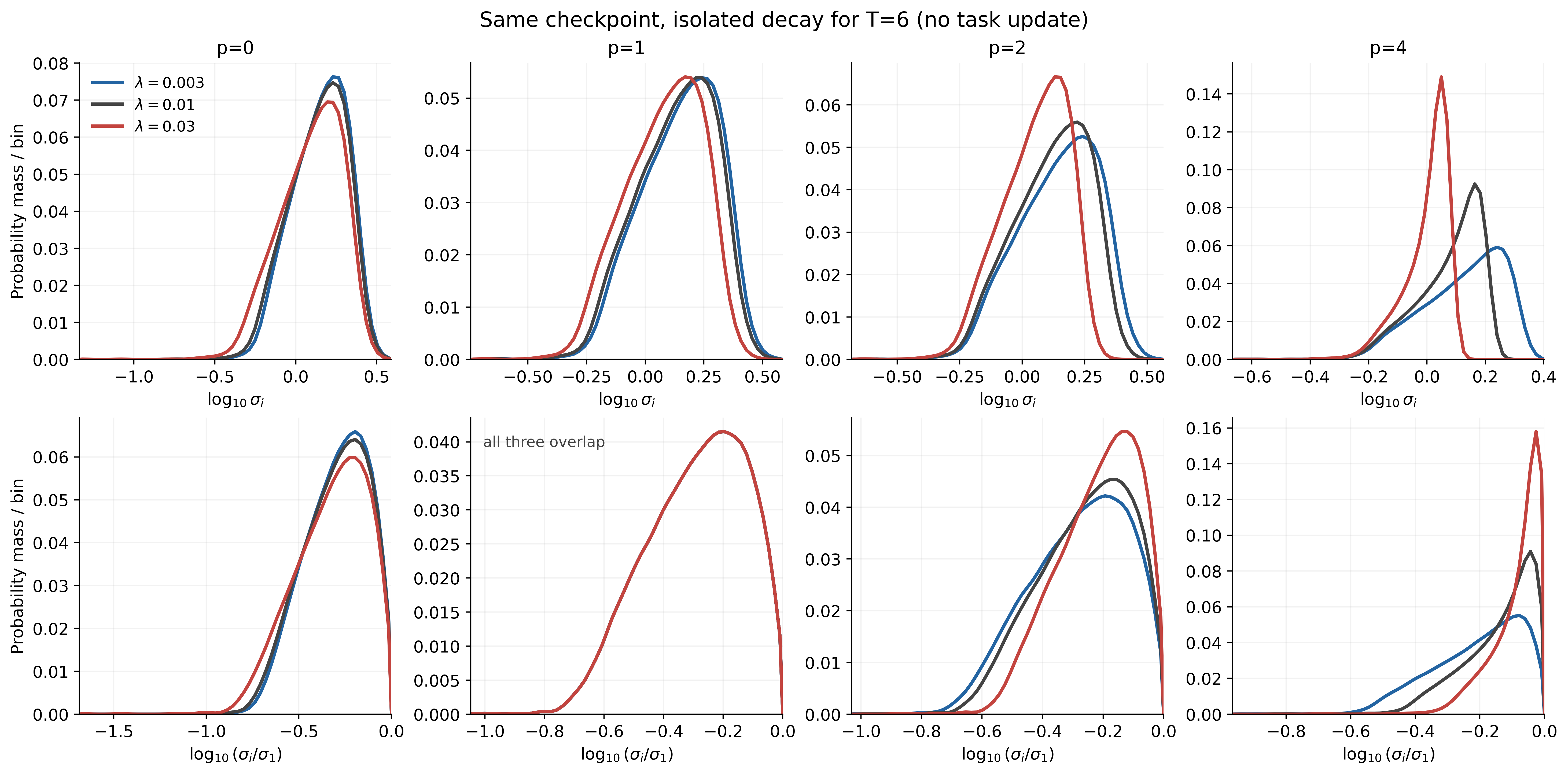
Figure 5. Analytic decay from the same checkpoint, with no task updates, over the fixed duration indicated in the plot. Columns correspond to ; rows show absolute and top-mode-normalized log spectra. Here is decay time, not the polar-iteration count in Algorithm 1.
At , increasing the coefficient translates the absolute log-spectrum while leaving the normalized distribution exactly unchanged. At , it also compresses the spread between the head and the bulk, most visibly at . The sharper normalized peak is another view of a flatter singular-value spectrum. At , the relative tail is instead suppressed.
After full training, increasing the coefficient from to gives the following changes in the MLP expansion matrices:
| Normalized log-spectrum distance | Mean stable-rank change | |
|---|---|---|
| 0 | 0.01955 | −5.6% |
| 1 | 0.00220 | −0.6% |
| 2 | 0.03131 | +11.4% |
| 4 | 0.06536 | +25.0% |
How the spectral distance is computed
Let be the th singular value of layer ‘s MLP expansion matrix divided by that matrix’s largest singular value. For eight layers with 512 modes each, define
Because the singular values are ordered and equally weighted, this is the average over layers of the first Wasserstein distance between their two log-spectrum distributions. It does not depend on histogram bins or smoothing. The distance gives the magnitude of the shape change; stable rank and the spectral curves indicate its direction.
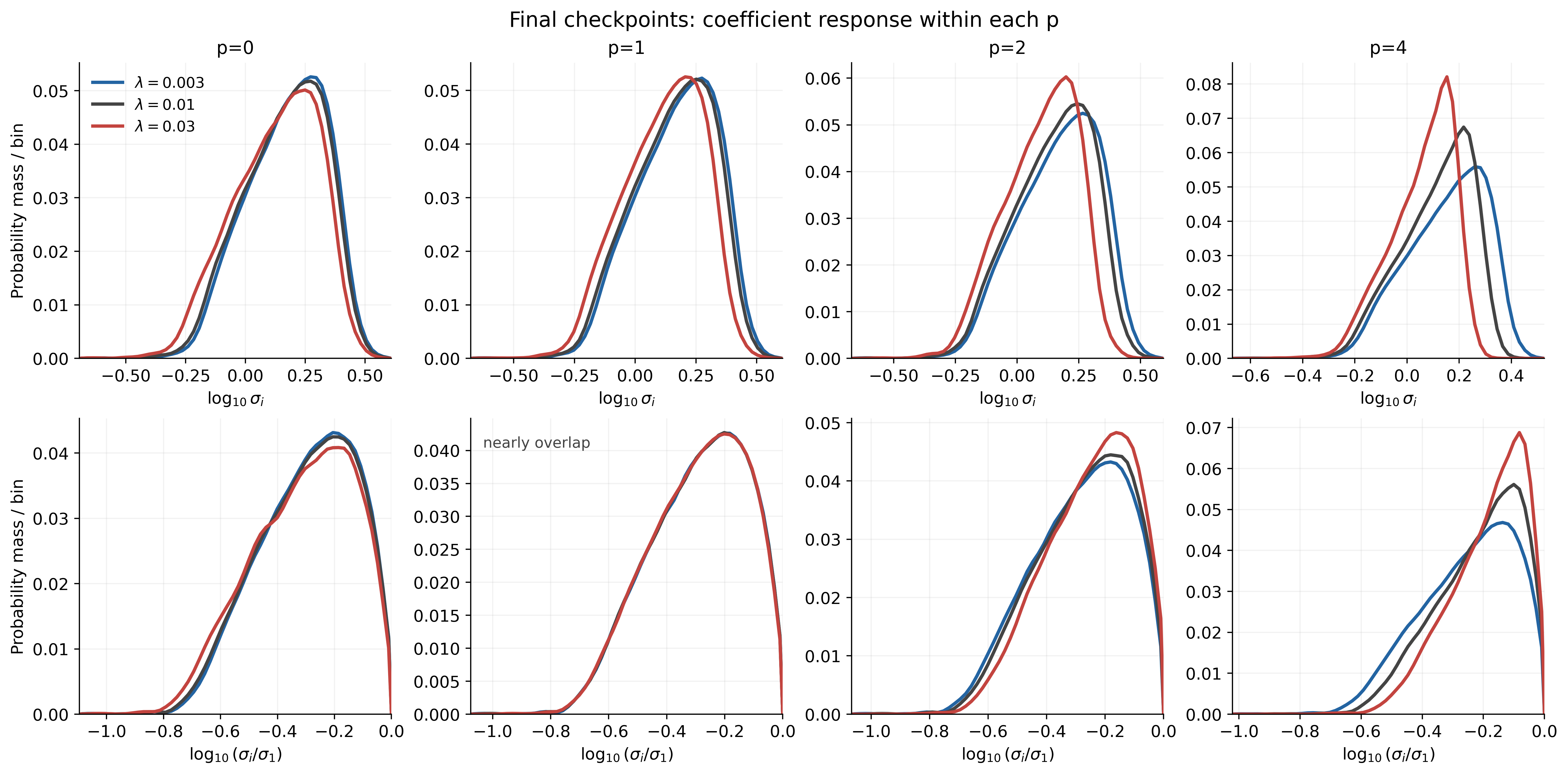
Figure 6. MLP expansion spectra at the end of full training, using the same coefficient values as Figure 5. Unlike the pure-decay comparison, these checkpoints have followed different task-and-decay trajectories. The normalized curves nearly overlap; the other powers show a larger shape response.
The trained MLP spectra retain the main pattern of the pure-decay comparison, but not its exact invariances. Ordinary WD produces only a small normalized-shape change here. That observation does not extend to every matrix family: in the same ordinary-WD sweep, mean Q and K stable ranks fall by about 7.7% and 14.4%, respectively. Once task updates are included, even ordinary WD can alter the learned spectral shape.
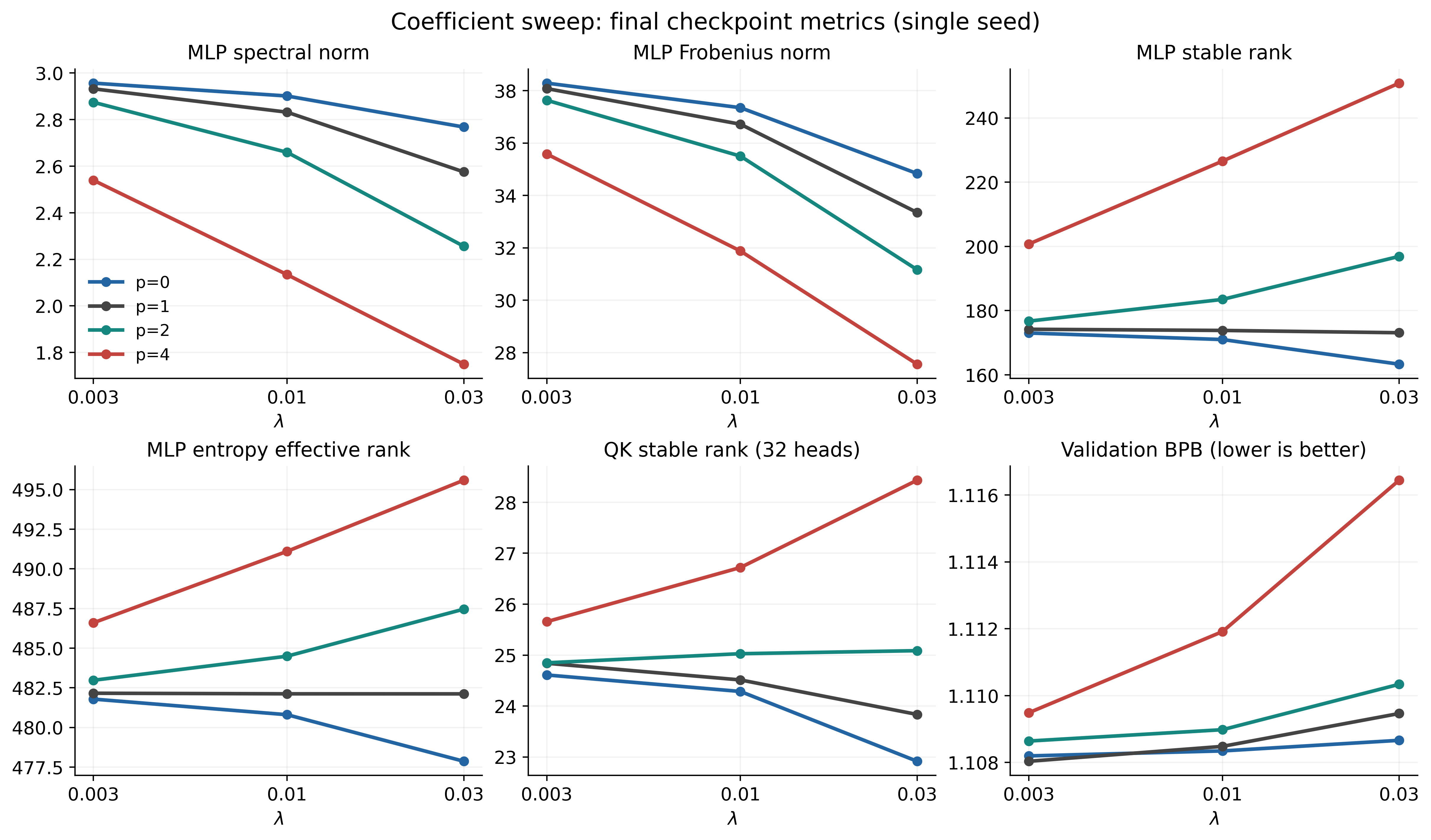
Figure 7. Final-checkpoint metrics from the coefficient sweep. Top row: MLP spectral norm, Frobenius norm, and stable rank. Bottom row: MLP entropy effective rank, QK-product stable rank across 32 heads, and validation bits per byte (BPB; lower is better).
At , increasing the coefficient from to raises mean MLP stable rank from about to , while lowering the spectral norm from about to . The Frobenius norm also falls. There is no contradiction: stable rank is , so it can rise when the leading singular value falls proportionally more than the Frobenius norm. The much smaller change in entropy effective rank suggests that the effect is chiefly a redistribution of relative magnitude, rather than the appearance of many new active dimensions.
The validation panel is equally important. Stronger decay produces the highest ranks in this sweep, but also worse BPB. The experiment establishes control over spectral geometry; it does not support maximizing rank as a training objective. Equal raw coefficients also do not give an equal-strength comparison across powers.
The remaining question is how to use this control within a training recipe. We turn to a case where the task-update geometry and the decay geometry can be adjusted separately.
4. Case study: Head-wise Muon and V spectral regularization
4.1 From head-wise to full-matrix V updates
Public reports for GLM-5, Kimi K3, and Qwen3.8-Next use head-wise Muon on query, key, and value weights (GLM-5 Team, 2026; Kimi Team, 2026; Qiu et al., 2026); DeepSeek-V4.1-Flash instead uses head-wise updates only for query and key (DeepSeek-AI, 2026).
Use H for head-wise updates and F for full-matrix updates, in Q/K/V order. HHH splits all three projections by head. HHF changes only V, applying Muon to the full matrix spanning all heads. Since Muon orthogonalizes task momentum, changing this grouping changes the task-update geometry. It does not directly make the weights or activations orthogonal.
Q/K determine where information is read from; V supplies the content being read and aggregated (Vaswani et al., 2017). Whether V heads learn complementary content features therefore deserves separate consideration. Head-wise polar shapes each momentum block separately, while full-matrix polar processes the entire V momentum jointly, including directional overlap across heads. This suggests a natural interpretation of HHF: joint updates may help the heads make fuller use of the available representation space. The learned representations change, while the architecture and parameter count remain the same.
We first compare HHH with HHF. We then keep the HHF update rule and add spectral decay to V, asking whether a separate adjustment to its weight spectrum helps.
4.2 Keeping the update rule, adjusting V decay
We retain ordinary WD and add a term to the full V weight:
The implementation uses LR-coupled coefficients: both and multiply the current learning rate . The definitions of and above translate this convention into our notation. The ideal decay direction is the gradient of . In an isolated step that does not cross zero, mode has relative shrinkage
The ordinary term shrinks every mode by the same fraction; the term adds pressure in proportion to its singular value. This changes the regularization while leaving the Muon update rule in place.
We compute the added term from the pre-update weight as , approximating the polar factor with Polar Express (Amsel et al., 2026). The comparison HHH → HHF → HHF + is between separate training runs, not successive stages of one run. Keeping the update rule fixed also does not mean that the realized task updates stay identical once the trajectories diverge.
Training protocol and coefficient sweeps
The HHH, HHF, and selected runs share the implementation, initialization, and ordered data stream. The model has 12 layers, width 768, and head dimension 128. Sequence length is 4096, global batch is 524,288 tokens, and seed is 42. Training lasts 16,204 steps, or 8,495,562,752 tokens. The peak learning rate is 0.005, with 256 warmup steps followed by cosine decay to 0.1 of peak. Ordinary WD is 0.1. Validation uses 10,485,760 tokens, with 164 evaluations during training. Muon scale is (Liu et al., 2025), with dimensions taken from the original full projection.
For HHF, the added coefficient ranges from to , with more points near . The control includes and a fine sweep over –. At , the extra term is ordinary WD, making V’s total coefficient . Coefficients across powers are not matched for decay strength.
4.3 Validation gains and their relation to rank
Final validation NLL is for HHH, for HHF, and for the selected HHF + run. Moving from HHH to HHF changes the V task-update scope. Adding decay then improves on the HHF control by about , at .
The two HHF trajectories have very similar overall V weight RMS, and the added spectral step is much smaller than the task step. This is a weak regularizer acting throughout training, not a decay-dominated regime. Pure-decay analysis describes the bias of the extra term; its effect on loss comes from its interaction with task updates.
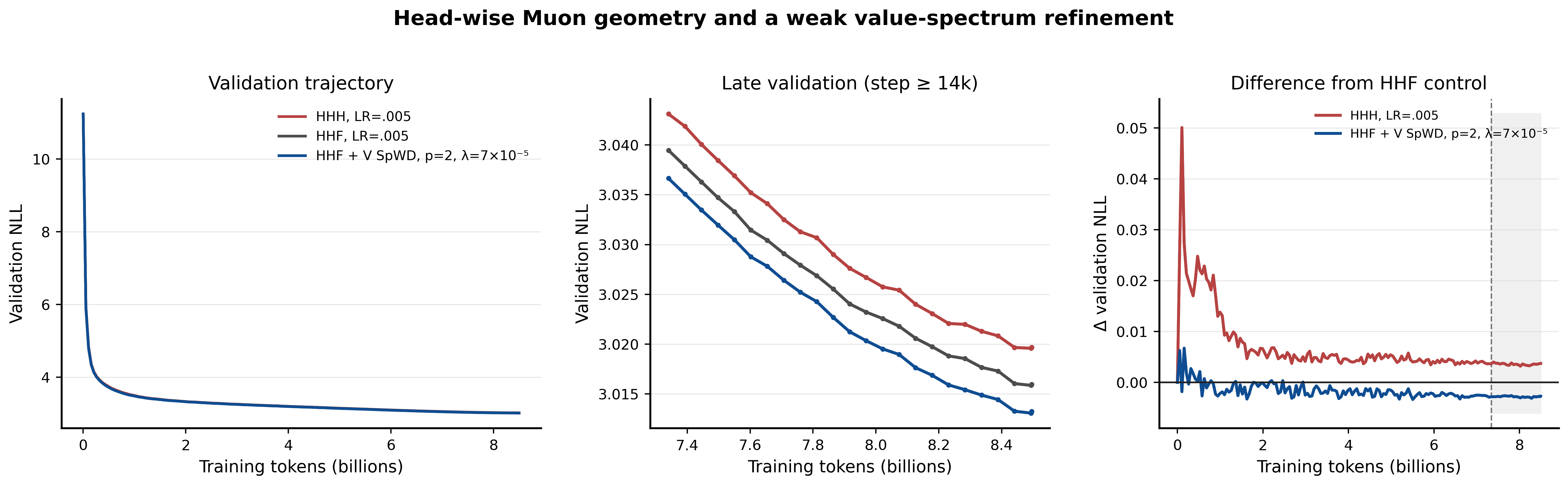
Figure 8. HHH, HHF, and the selected HHF + full-V run from a common initialization. Left: full validation trajectories. Middle: the late-training window, at steps . Right: validation NLL relative to the HHF control, with that window shaded.
The full-scale curves nearly overlap, while the difference plot reveals persistent differences throughout the late-training window: HHF has lower validation loss than HHH, and adding decay improves it further.
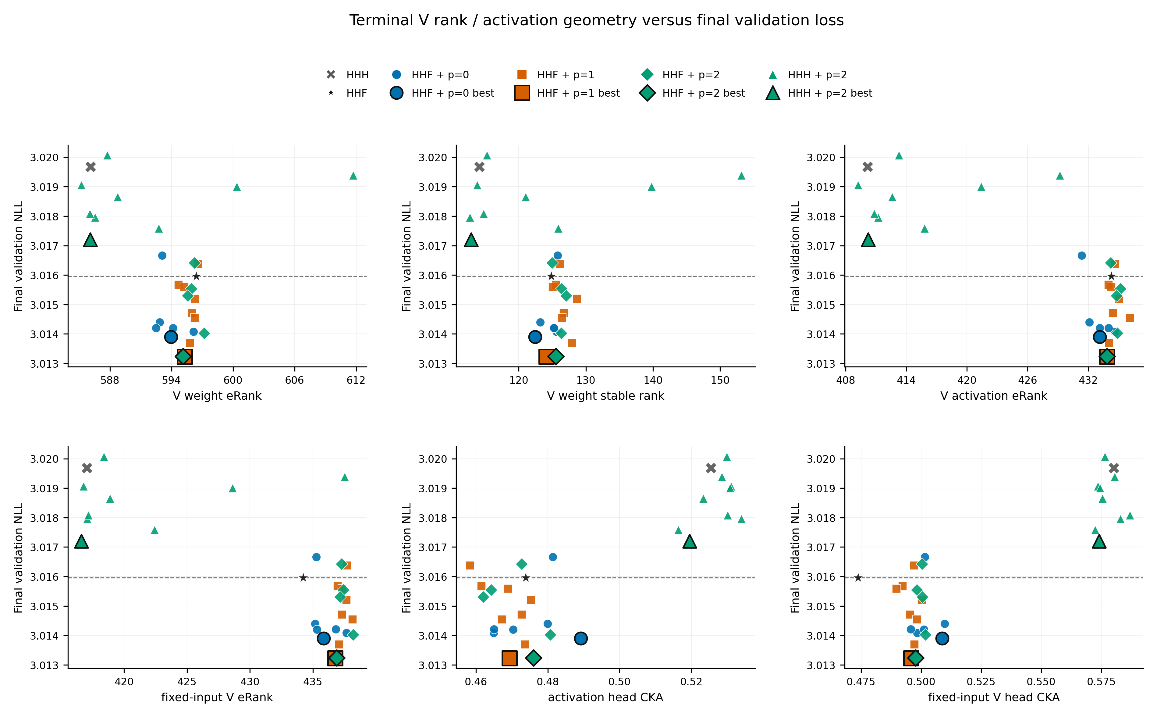
Figure 9. Endpoint V geometry versus final validation NLL. Top row: weight eRank, weight stable rank, and actual activation eRank. Bottom row: fixed-input activation eRank, actual activation head CKA, and fixed-input head CKA. Ranks are not divided by dimension. Crosses and stars denote HHH and HHF; circles, squares, and diamonds denote the HHF sweeps; triangles denote HHH + . Heavy outlines mark the best point in each family. The dashed line is the HHF control loss.
From HHH to HHF, the distinction is clearer in V’s content representations. Actual activation eRank rises from about to , while cross-head CKA falls from about to . The fixed-input comparison likewise shows higher eRank and lower CKA. On the sampled inputs, HHF’s content responses span more effective directions and show less statistical overlap across heads. This is consistent with one possible explanation: full-V updates help the heads learn more complementary content features, reducing representation redundancy that may arise with head-wise updates. The fixed-input result also locates a difference in the V map itself, rather than attributing it entirely to changes upstream.
The plot offers another interesting comparison: some HHH + runs have higher weight eRank or stable rank than HHF, yet worse loss. HHF’s advantage is therefore more naturally interpreted through the content representations it learns. The effective directions in the joint activations, complementarity across heads, and the task’s use of those directions together offer a fuller explanation than weight rank alone. This also connects to recent Muon discussions of the relationship between spectral shape and task performance (Goyal & Ramkumar, 2026).
Within HHF, spectral decay offers finer control over the representations. Actual activation-eRank points form an almost vertical cloud: similar effective dimensions accompany different losses. Compared with the HHF control, the best point has slightly lower weight eRank, nearly unchanged actual activation eRank, modestly higher fixed-input eRank, and higher values of both CKAs. Similar effective dimensions can therefore accommodate different ways of organizing content and different task outcomes.
The best control also lies very close to the best point. This makes V regularization an especially useful component to tune separately: adjusting ordinary decay already helps, while spectral powers additionally let us choose how shrinkage is distributed across modes. The more interesting question is how to align that extra freedom with the needs of the content representations.
How ranks and CKA are measured
Weight ranks are computed on the full V matrix. Actual activation ranks use each layer’s centered, sampled V output, and therefore include the checkpoint’s own upstream representations. Fixed-input measurements apply each checkpoint’s V weights to the HHF control’s layer inputs. All plotted ranks are averaged over 12 layers.
For two centered head outputs , linear CKA is
We average the 15 pairs among six heads, then average over 12 layers (Kornblith et al., 2019). Higher CKA means more similar representations under this statistic. The fixed-input comparison holds the sampled inputs constant, helping distinguish changes in the V map from changes upstream.
We conjecture that full-V updates and spectral decay can improve effective representational capacity in complementary ways. The former processes update directions jointly across heads, helping them learn complementary content; the latter adjusts relative mode magnitudes, allowing task updates to make fuller use of the representation space. For example, suppresses overly dominant modes while preserving the relative contribution of the bulk and tail, potentially letting the same parameters support richer effective representations. This capacity involves both the number of effective directions and how information is distributed across heads. The next experiment asks how much these internal structures can differ when final validation loss is almost the same.
5. Case study: nearly the same pretraining loss, different rank geometry
5.1 Choosing a spectral preference for each module
We compare ordinary WD with an asymmetric recipe that assigns different powers to Attention and MLP weights, then look for runs with nearly matching final validation loss.
Attention mixes information across tokens; the MLP transforms features within each token. This suggests testing different spectral preferences: for Attention, to put relatively more pressure on weak modes, and for the MLP, to reduce the dominance of large modes. The experiment is motivated by low-rank attention analysis and module-wise decay allocation (He et al., 2025; Kobayashi et al., 2024), rather than an assumption that either module has a universally optimal rank.
Both families use Muon for matrix updates and the independent-coefficient convention: multiplies both branches, but and receive no additional factor of . There is no extra ordinary-WD term. These coefficients therefore cannot be compared numerically with the LR-coupled coefficients in Section 4.
The baseline uses ; the asymmetric recipe uses . Here and denote Attention and MLP. Both families are allowed to tune their module-wise coefficients over the same grid of base learning rates and decay coefficients:
This gives configurations per family, or 54 in total. Below, we compare the two runs with the closest final validation losses. They share the model, initialization, seed, ordered data stream, and validation data. Both train for 7,268 steps with :
| Run | Attention | MLP | Loss before LR cooldown | Final validation loss |
|---|---|---|---|---|
| Ordinary-WD baseline | 3.107320711 | 3.000562422 | ||
| Asymmetric | 3.109563260 | 3.000577086 |
The final losses differ by approximately nats.
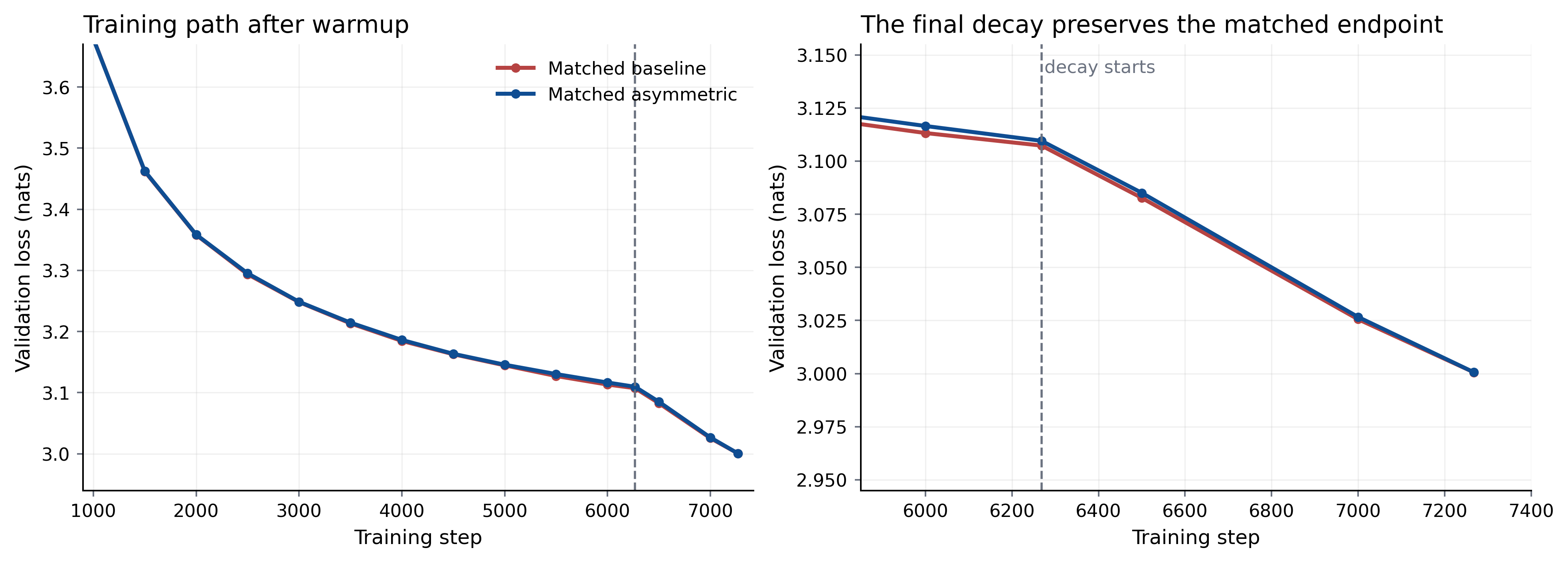
Figure 10. Validation trajectories of the selected ordinary-WD and asymmetric runs. Left: training after warmup. Right: a close-up around the final learning-rate cooldown, marked by the dashed line. Both runs finish at step 7,268.
The trajectories are close well before the final point. Their loss gap is about nats before cooldown and narrows further by the end. Similar fitting outcomes make the internal-geometry comparison below especially interesting.
5.2 Similar loss leaves room for different internal geometry
| Weight or product metric | Ordinary baseline | Asymmetric |
|---|---|---|
| Attention spectral norm | 3.3083 | 4.6478 |
| Attention stable rank | 89.90 | 78.75 |
| Attention entropy eRank | 587.03 | 565.05 |
| MLP spectral norm | 6.1150 | 4.1062 |
| MLP stable rank | 184.28 | 258.61 |
| MLP entropy eRank | 729.97 | 743.00 |
| QK product stable rank | 15.57 | 17.06 |
In this pair, asymmetric decay produces more concentrated Attention weight spectra and higher-stable-rank MLP spectra, broadly matching the intended preferences. “Attention” in these weight statistics refers to the projection weights, not the post-softmax attention maps. The QK-product stable rank nevertheless rises. A product’s spectrum depends on the alignment of its factors’ singular vectors as well as their singular values, so lower factor ranks need not translate into a lower product stable rank.
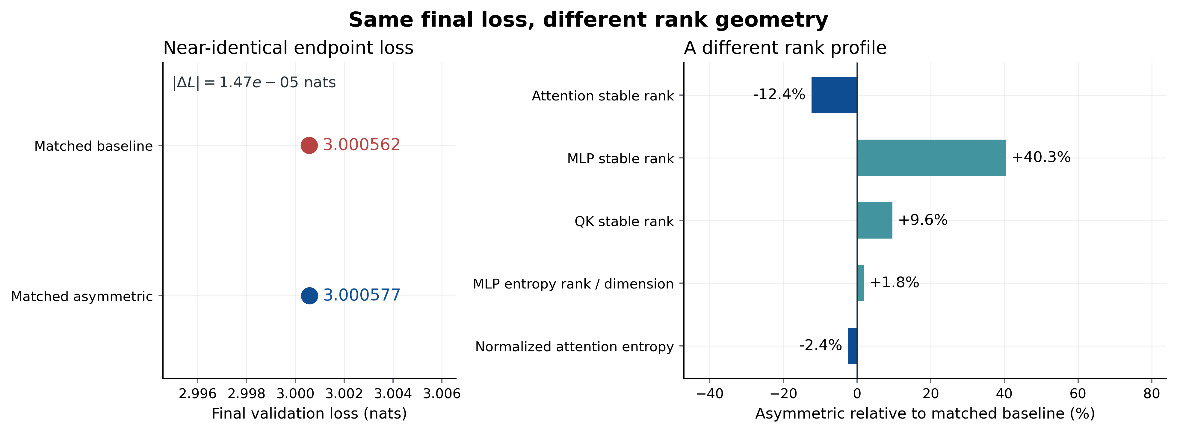
Figure 11. Nearly matched final validation loss, different endpoint geometry. The right panel reports changes relative to the ordinary-WD baseline: Attention weight stable rank, MLP weight stable rank, QK-product stable rank, dimension-normalized MLP eRank, and normalized attention entropy.
MLP stable rank increases by 40.3%, while its dimension-normalized eRank increases by only 1.8%. These measures emphasize different features: the former is particularly sensitive to the leading singular value; the latter summarizes the distribution across all modes. The result is better described as a substantial change in relative spectral concentration than as a 40% increase in representational dimension.
The accompanying forward-pass measurements also differ. From ordinary WD to asymmetric decay, normalized attention entropy falls from to , while mean maximum attention probability rises from to . Q activation RMS rises from to , and MLP output RMS falls from to . Thus, nearly equal average validation loss can coexist with different attention distributions and internal scales.
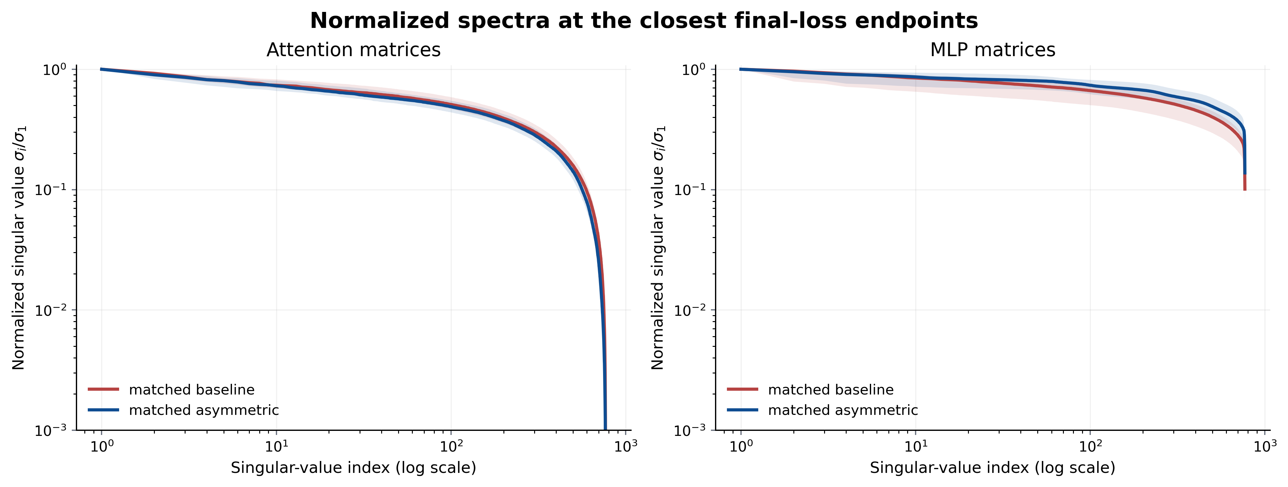
Figure 12. Normalized weight spectra at the selected endpoints. Attention projections become more concentrated, while MLP spectra become flatter. The norm measurements in the table give the corresponding absolute-scale comparison.
The logarithmic horizontal axis emphasizes the leading modes and compresses much of the remaining spectrum. A modest visual separation across many middle and tail modes can still matter for stable rank, which sums over indices without logarithmic weighting. The normalized curves also hide an important scale difference: Attention spectral norm is larger in the asymmetric run, whereas MLP spectral norm is smaller.
These runs retain different internal spectra and activation statistics at nearly the same pretraining loss. Spectral decay thus offers an interesting form of control: exploring different information allocations and representation structures at similar fitting performance, then comparing how they behave in transfer, fine-tuning, and robustness.
6. A related extension: spectral projection in the decay branch
A power law changes shrinkage across the whole spectrum. We can also ask which modes should receive it. Recent work uses a shifted Gram matrix and a symmetric matrix sign to select momentum subspaces above or below a threshold (Goyal & Ramkumar, 2026). Applying the same construction to weights gives a band-selective decay rule without changing the task optimizer.
Constructing the projector. Take with , and choose a singular-value threshold that is not equal to any singular value. Set and
Here is the identity. The symmetric matrix sign keeps eigenvectors and replaces each eigenvalue by its sign: if , then . Since , its positive and negative eigenspaces correspond exactly to modes above and below the threshold. and project onto these subspaces.
The source paper applies this operation to momentum , constructing and from . With , the two task directions are
The selected subspace receives the polar direction; the other retains raw momentum. For weight decay, the analogous mixed rule applies in one subspace and ordinary WD in the other:
Alternatively, leave the unselected subspace unchanged by decay. To distinguish this from the mixed rule, write
Computing the projector without an SVD. Normalize the symmetric shifted matrix as , then apply the convergent fifth-degree Newton–Schulz iteration
This odd polynomial preserves eigenvalue signs and drives nonzero modes toward . Forming allows to be reused. Modes near the threshold correspond to eigenvalues near zero and take longer to resolve; the source paper uses 20 FP32 iterations for both sign calls in NanoGPT (Goyal & Ramkumar, 2026). At a finite iteration count, the resulting matrices are approximate projectors, not exact binary selectors. Accuracy depends on the spectral gap around the threshold.
The resulting mode-wise update. For an isolated top-selective step, expressed in the current singular basis and small enough to keep the mode coefficients nonnegative,
In continuous time, the corresponding pure-decay law is . The threshold selects the modes, the power sets their shrinkage law, and the coefficient sets its strength. Recomputing the projectors from the current also lets us assign separate powers and coefficients to the two subspaces. For ,
Setting one coefficient to zero restricts decay to one band. Setting both powers to one and both coefficients equal recovers ordinary WD. For , use and left-multiply by the corresponding projectors, as in Section 3.2.
This extension separates two decisions: which modes to regularize, and how strongly shrinkage should depend on their size. Its usefulness in training still needs to be tested; the construction itself only specifies the decay rule.
7. Closing thoughts
Ordinary WD scales all singular values equally in an isolated step. WD changes that rule with one exponent: puts relatively more pressure on weak modes, while puts more pressure on strong ones. The linear model makes the effect exact; the eight-layer Transformer shows that it can remain visible after task-driven training.
The case studies show concrete uses for this control. In the V experiment, full-matrix updates learn more spread-out content representations with less cross-head overlap, and further regularization tuning improves the default HHF recipe. In the asymmetric experiment, nearly matching validation loss still accompanies markedly different weight spectra and activation statistics. These results invite a further question: how should mode magnitudes and roles be allocated to make fuller use of a model’s effective representational capacity?
The useful addition is a way to specify and test spectral preferences rather than leaving them entirely to the optimizer and scalar decay. Powers, coefficients, module allocation, and band selection offer progressively finer choices. Which ones help depends on the task and training regime. Stage-dependent spectral regularization in ORCA (Y. Liu et al., 2026) and quantization-oriented spectral decay in S²D (Chavan et al., 2026) suggest concrete settings in which to study that question.
Spectrum shaping may also serve as a tool for training stability. Spectral-norm reparameterization has been used to mitigate attention entropy collapse and improve Transformer training stability (Zhai et al., 2023). We conjecture that or spectral-band selection could target excessively amplified modes, helping control spectral-norm growth, reduce loss spikes, and widen the range of stable learning rates.
Weight decay need not shrink every mode in the same proportion. Choosing a different shrinkage law gives us control over the spectrum; whether that control is useful has to be answered by the task.
- Amsel, N., Persson, D., Musco, C., & Gower, R. M. (2026). The Polar Express: Optimal Matrix Sign Methods and their Application to the Muon Algorithm. The Fourteenth International Conference on Learning Representations. https://openreview.net/forum?id=yRtgZ1K8hO back: 1, 2, 3
- Andriianov, D., Veprikov, A., & Beznosikov, A. (2026). Spectral Weight Decay: Inducing Low-Rank Structure in Neural Network Weights. https://arxiv.org/abs/2610.11730
- Cai, J.-F., Candès, E. J., & Shen, Z. (2010). A Singular Value Thresholding Algorithm for Matrix Completion. SIAM Journal on Optimization, 20(4), 1956–1982. 10.1137/080738970 back: 1, 2, 3, 4
- Chavan, A., Lele, N., Bamba, U., Dayal, S., Raghunathan, A., & Gupta, D. (2026). S2D: Selective Spectral Decay for Quantization-Friendly Conditioning of Neural Activations. https://arxiv.org/abs/2602.14432
- DeepSeek-AI. (2026). DeepSeek-V4.1-Flash: Pushing the Limits of KV Cache Compression. arXiv Preprint arXiv:2609.19969. https://arxiv.org/abs/2609.19969
- Duchi, J., Hazan, E., & Singer, Y. (2011). Adaptive Subgradient Methods for Online Learning and Stochastic Optimization. Journal of Machine Learning Research, 12(61), 2121–2159. http://jmlr.org/papers/v12/duchi11a.html
- Eckart, C., & Young, G. (1936). The approximation of one matrix by another of lower rank. Psychometrika, 1, 211–218. 10.1007/BF02288367
- Ghiasi, A., Shafahi, A., & Ardekani, R. (2023). Improving Robustness with Adaptive Weight Decay. Thirty-Seventh Conference on Neural Information Processing Systems. https://openreview.net/forum?id=ajnThDhuq6
- GLM-5 Team. (2026). GLM-5: From Vibe Coding to Agentic Engineering. arXiv Preprint arXiv:2602.15763. https://arxiv.org/abs/2602.15763
- Goyal, V., & Ramkumar, R. (2026). Spectrally Targeted Muon. https://arxiv.org/abs/2610.10965 back: 1, 2, 3
- Gupta, V., Koren, T., & Singer, Y. (2018). Shampoo: Preconditioned Stochastic Tensor Optimization. Proceedings of the 35th International Conference on Machine Learning. https://proceedings.mlr.press/v80/gupta18a.html
- He, D., Tu, S., Jaiswal, A., Shen, L., Yuan, G., Liu, S., & Yin, L. (2025). AlphaDecay: Module-wise Weight Decay for Heavy-Tailed Balancing in LLMs. https://arxiv.org/abs/2506.14562 back: 1, 2
- Higham, N. J. (1986). Computing the Polar Decomposition—with Applications. SIAM Journal on Scientific and Statistical Computing, 7(4), 1160–1174. 10.1137/0907079
- Higham, N. J. (2002). Accuracy and Stability of Numerical Algorithms (2nd ed.). 10.1137/1.9780898718027
- Hoerl, A. E., & Kennard, R. W. (1970). Ridge Regression: Biased Estimation for Nonorthogonal Problems. Technometrics, 12(1), 55–67. 10.1080/00401706.1970.10488634
- Jordan, K., Jin, Y., Boza, V., You, J., Cesista, F., Newhouse, L., & Bernstein, J. (2024). Muon: An optimizer for hidden layers in neural networks. https://kellerjordan.github.io/posts/muon/ back: 1, 2
- Kessy, A., Lewin, A., & Strimmer, K. (2018). Optimal Whitening and Decorrelation. The American Statistician, 72(4), 309–314. 10.1080/00031305.2016.1277159
- Kimi Team. (2026). Kimi K3: Open Frontier Intelligence. arXiv Preprint arXiv:2607.24653. https://arxiv.org/abs/2607.24653
- Kingma, D. P., & Ba, J. (2015). Adam: A Method for Stochastic Optimization. International Conference on Learning Representations. https://arxiv.org/abs/1412.6980
- Kobayashi, S., Akram, Y., & von Oswald, J. (2024). Weight Decay Induces Low-Rank Attention Layers. Advances in Neural Information Processing Systems 37. https://arxiv.org/abs/2410.23819 back: 1, 2
- Kornblith, S., Norouzi, M., Lee, H., & Hinton, G. (2019). Similarity of Neural Network Representations Revisited. Proceedings of the 36th International Conference on Machine Learning, 97, 3519–3529. https://proceedings.mlr.press/v97/kornblith19a.html
- Krogh, A., & Hertz, J. A. (1991). A Simple Weight Decay Can Improve Generalization. Advances in Neural Information Processing Systems, 4. https://papers.neurips.cc/paper_files/paper/1991/hash/8eefcfdf5990e441f0fb6f3fad709e21-Abstract.html
- Lewis, A. S. (1995). The Convex Analysis of Unitarily Invariant Matrix Functions. Journal of Convex Analysis, 2(1–2), 173–183. 10.68381/jca02012 back: 1, 2, 3
- Liu, J., Su, J., Yao, X., Jiang, Z., Lai, G., Du, Y., Qin, Y., Xu, W., Lu, E., Yan, J., Chen, Y., Zheng, H., Liu, Y., Liu, S., Yin, B., He, W., Zhu, H., Wang, Y., Wang, J., … Yang, Z. (2025). Muon is Scalable for LLM Training. https://arxiv.org/abs/2502.16982
- Liu, Y., Jiang, B., Hou, L., Tao, X., Wan, P., Lin, Z., & Fang, C. (2026). ORCA: The Annealed Spectral Conditioning Optimizer for Faster, Better LLM Training. https://arxiv.org/abs/2610.06116
- Loshchilov, I., & Hutter, F. (2019). Decoupled Weight Decay Regularization. International Conference on Learning Representations. https://openreview.net/forum?id=Bkg6RiCqY7 back: 1, 2
- Martens, J., & Grosse, R. (2015). Optimizing Neural Networks with Kronecker-factored Approximate Curvature. Proceedings of the 32nd International Conference on Machine Learning, 2408–2417. https://proceedings.mlr.press/v37/martens15.html
- Nakamura, K., & Hong, B.-W. (2019). Adaptive Weight Decay for Deep Neural Networks. https://arxiv.org/abs/1907.08931
- Parikh, N., & Boyd, S. (2014). Proximal Algorithms. Foundations and Trends in Optimization, 1(3), 123–231. https://web.stanford.edu/~boyd/papers/prox_algs.html back: 1, 2
- Qiu, Z., Wang, Z., Li, X., Li, Y., Xu, Y., Wang, Y., Zhang, H., Men, R., Mao, B., Zhang, C., Zhou, F., Luo, H., Huang, H., Lian, H., Huang, H., Chen, H., Zhang, J., Xu, J., Wang, J., … Liu, D. (2026). On the Design of Qwen3.8-Next Architecture: Evaluation, Efficiency, and Training Stability. https://arxiv.org/abs/2608.30320
- Roy, O., & Vetterli, M. (2007). The Effective Rank: A Measure of Effective Dimensionality. 15th European Signal Processing Conference, 606–610. https://eurasip.org/Proceedings/Eusipco/Eusipco2007/Papers/a5p-h05.pdf back: 1, 2, 3
- Sanyal, A., Torr, P. H. S., & Dokania, P. K. (2020). Stable Rank Normalization for Improved Generalization in Neural Networks and GANs. International Conference on Learning Representations. https://openreview.net/forum?id=H1enKkrFDB
- Shannon, C. E. (1948). A Mathematical Theory of Communication. The Bell System Technical Journal, 27(3), 379–423. 10.1002/j.1538-7305.1948.tb01338.x
- Srebro, N., Rennie, J. D. M., & Jaakkola, T. S. (2004). Maximum-Margin Matrix Factorization. Advances in Neural Information Processing Systems, 17, 1329–1336. https://proceedings.neurips.cc/paper/2004/hash/e0688d13958a19e087e123148555e4b4-Abstract.html
- Sutskever, I., Martens, J., Dahl, G., & Hinton, G. (2013). On the importance of initialization and momentum in deep learning. Proceedings of the 30th International Conference on Machine Learning, 28(3), 1139–1147. https://proceedings.mlr.press/v28/sutskever13.html
- Tang, X., Zhang, H., Cao, Y., & Zou, D. (2025). Understanding the Generalization of Stochastic Gradient Adam in Learning Neural Networks. Advances in Neural Information Processing Systems, 38. 10.52202/085713-0612
- Tikhonov, A. N., & Arsenin, V. Y. (1977). Solutions of Ill-Posed Problems. Winston. https://catalog.library.tamu.edu/Record/in00000360774/Details
- van Laarhoven, T. (2017). L2 Regularization versus Batch and Weight Normalization. https://arxiv.org/abs/1706.05350
- Vaswani, A., Shazeer, N., Parmar, N., Uszkoreit, J., Jones, L., Gomez, A. N., Kaiser, Ł., & Polosukhin, I. (2017). Attention Is All You Need. Advances in Neural Information Processing Systems, 30. https://arxiv.org/abs/1706.03762 back: 1, 2
- Vyas, N., Morwani, D., Zhao, R., Kwun, M., Shapira, I., Brandfonbrener, D., Janson, L., & Kakade, S. (2025). SOAP: Improving and Stabilizing Shampoo using Adam. https://arxiv.org/abs/2409.11321
- Watson, G. A. (1992). Characterization of the subdifferential of some matrix norms. Linear Algebra and Its Applications, 170, 33–45. 10.1016/0024-3795(92)90407-2 back: 1, 2, 3
- Wen, K., Dang, X., Lyu, K., Ma, T., & Liang, P. (2026). Fantastic Pretraining Optimizers and Where to Find Them II: Hyperball Optimization. https://arxiv.org/abs/2606.16899
- Zhai, S., Likhomanenko, T., Littwin, E., Busbridge, D., Ramapuram, J., Zhang, Y., Gu, J., & Susskind, J. M. (2023). Stabilizing Transformer Training by Preventing Attention Entropy Collapse. Proceedings of the 40th International Conference on Machine Learning, 202, 40770–40803. https://proceedings.mlr.press/v202/zhai23a.html back: 1, 2
- Zhang, G., Wang, C., Xu, B., & Grosse, R. (2019). Three Mechanisms of Weight Decay Regularization. International Conference on Learning Representations. https://arxiv.org/abs/1810.12281
- Zou, D., Cao, Y., Li, Y., & Gu, Q. (2023). Understanding the Generalization of Adam in Learning Neural Networks with Proper Regularization. International Conference on Learning Representations. https://openreview.net/forum?id=iUYpN14qjTF